Some Gaussians hidden in uniform measures…

Consider a vector ${\theta\sim\textsf{N}(0, {\textrm{I}}/N)}$ where ${\theta \in {\mathbb R}^N}$ . It is often claimed that this distribution is “very close”, in the limit of large ${N}$ , to that of the uniform measure on the sphere ${S_N \subset {\mathbb R}^N}$ of unit radius. This is, in fact, not hard to see (informally) using a Chernoff bound argument. Firstly, let ${\theta_i}$ denote the ${i^{\mathrm{th}}}$ entry of ${\theta}$ . More precisely, the Chernoff argument yields the following inequalities:

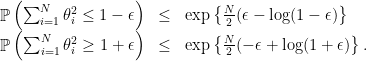
$\displaystyle \begin{array}{rcl} \mathop{\mathbb P}\left(\sum_{i=1}^N\theta_i^2 \le 1-\epsilon\right)&\le& \exp\left\{ \frac{N}{2}(\epsilon - \log(1-\epsilon) \right\} \\ \mathop{\mathbb P}\left(\sum_{i=1}^N\theta_i^2 \ge 1+\epsilon \right)&\le& \exp\left\{ \frac{N}{2}(-\epsilon + \log(1+\epsilon) \right\}. \end{array}$

The way to obtain this is pretty standard. For instance the first inequality can be obtained as:

$\displaystyle \begin{array}{rcl} \mathop{\mathbb P}\left(\sum_{i=1}^N\theta_i^2 \le 1-\epsilon\right)&=&\mathop{\mathbb P}\left[\exp(-\lambda \sum_{i=1}^N\theta_i^2) \ge \exp(-\lambda(1-\epsilon)) \right]\\ &\le& \mathop{\mathbb E}\left[ \exp(-\lambda\sum_{i=1}^N \theta_i^2) \right]\exp(\lambda(1-\epsilon)), \end{array}$

where ${\lambda\ge0}$ and the inequality is by Markov. Optimizing over ${\lambda}$ yields the result. This tells us that ${\lVert\theta\rVert^2}$ concentrates around the expected value of 1 at least to the extent of ${O(N^{-1/2 + \delta})}$ for a small constant ${\delta}$ . In fact one can do better than this using an exact large deviations calculation, which I will probably leave to another post.

Thus for large dimensions ${N}$ , the probability mass of the distribution ${\textsf{N}(0, {\textrm{I}}/N)}$ is concentrated in a shell of thickness ${O(N^{-1/2})}$ and mean radius 1, which intuitively, looks very much like ${S_N}$ . The question that interested me is how we can prove the converse: assuming ${\theta\sim U(S_N)}$ where ${U(S_N)}$ denotes the spherical measure on ${S_N}$ do the marginals of each entry, say ${\theta_1}$ look Gaussian? More precisely, let ${\mu_N}$ denote the measure of ${\sqrt N \theta_1}$ on ${({\mathbb R}, \mathcal{B})}$ . Then, does ${\mu_N}$ converge weakly to ${\textsf{N}(0, 1)}$ ? This is, in fact, true and is an old result due to Borel in his (book/treatise) “Introduction géometrique à quelques théorie physiques”. I will sketch a simple argument via characteristic functions.

The function 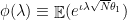${\phi(\lambda) \equiv \mathop{\mathbb E}(e^{\iota\lambda\sqrt N \theta_1})}$ is the characteristic function of ${\sqrt N \theta_1 \sim \mu_N}$ , where ${\iota = \sqrt{-1}}$ . We can compute this integral explicitly. The formula for the “area” of an ${N}$ -dimensional spherical cap as given (here) is:

$\displaystyle \begin{array}{rcl} A &=& \frac{1}{2}A_N I_{2h-h^2}\left( \frac{N-1}{2}, \frac{1}{2} \right), \end{array}$

where ${A_N}$ is the surface area of ${S_N}$ , ${h}$ is the depth and ${I_{2h-h^2}(\cdot, \cdot)}$ is the normalized incomplete beta function. Differentiating this, dividing by ${A_N}$ and noting that ${h \equiv 1 - \theta_1}$ , we can compute the characteristic function as the following integral:

$\displaystyle \begin{array}{rcl} \phi(\lambda) &=& B\left( \frac{n-1}{2}, \frac{1}{2} \right)^{-1} \int_{-1}^1 e^{\iota\lambda\sqrt N \theta_1}(1-\theta_1)^{(N-3)/2}\mathrm{d}\theta_1, \end{array}$

where ${B(\cdot, \cdot)}$ is the beta function. To do the above, we have to take care of a few sign conventions, which I have omitted. Now, 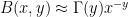${B(x, y) \approx \Gamma(y)x^{-y}}$ for fixed ${y}$ and large ${x}$ by Stirling’s approximation. With this and a change of variables ${y \equiv \sqrt N \theta_1}$ , we obtain:

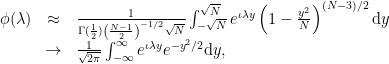
$\displaystyle \begin{array}{rcl} \phi(\lambda) &\approx& \frac{1}{\Gamma(\frac{1}{2}) \left( \frac{N-1}{2} \right)^{-1/2}\sqrt{N}} \int_{-\sqrt N}^{\sqrt N} e^{\iota\lambda y}\left( 1-\frac{y^2}{N} \right)^{(N-3)/2}\mathrm{d}y \\ &\rightarrow& \frac{1}{\sqrt{2\pi}} \int_{-\infty}^\infty e^{\iota \lambda y} e^{-y^2/2}\mathrm{d}y, \end{array}$

by dominated convergence. The last limit is precisely what we require, namely the characteristic function 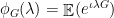${\phi_G(\lambda) = \mathop{\mathbb E}(e^{\iota\lambda G})}$ where ${G\sim\textsf{N}(0,1)}$ . The rest follows from Lévy’s continuity theorem.

There are significant improvements to this result. Diaconis and Freedman prove that this holds for all low-dimensional marginals, even in the sense of variation distance. More precisely, let ${\theta_k \in {\mathbb R}^k}$ denote the restriction of ${\theta}$ to the first ${k}$ entries. They give a sharp bound on the variation distance between the law of ${\sqrt{N}\theta_k}$ and ${\textsf{N}(0, {\textrm{I}}_k)}$ . Interesting generalizations include this result by D’Aristotile, Diaconis and Newman which says that 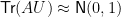${\mathop{\textsf{Tr}}(AU) \approx \textsf{N}(0, 1)}$ when ${U}$ is a orthogonal matrix of size ${N\times N}$ chosen uniformly at random, and ${\mathop{\textsf{Tr}}(AA^\textsf{T}) = N}$ , and others which state that even a “small” submatrix of ${U}$ behaves as though its entries were iid standard normals.

I am sure I have barely scratched the surface here, but it is clear that many (and sometimes intuitively plausible) approximations of this kind are actually fairly accurate even rigorously.

UPDATE (04/05/13): Thanks to Jiantao Jiao for some corrections above.

This entry was posted on February 5, 2013 at 2:44 PM and is filed under Uncategorized. You can follow any responses to this entry through the RSS 2.0 feed. You can leave a response, or trackback from your own site.

Theory and More